10 Programs Every Machine Learning Engineer Must Know How to Write

There’s a quiet line that separates two kinds of machine learning engineer. On one side are people who can call model.fit(X, y) and read the accuracy score. On the other are people who know what .fit() actually did — which knob it turned, why the loss went down, and what will break when the data shifts. The second group debugs faster, designs better experiments, and doesn’t panic when a model behaves strangely in production.

The fastest way to cross that line isn’t reading more theory. It’s writing ten small programs at least once, by hand, without leaning on a library to do the interesting part. Each of these takes an afternoon. Together they build the mental model that makes every framework you touch afterward feel transparent instead of magical.

This isn’t a list of tools to install. It’s a list of things you should be able to implement from an empty file — because implementing them is what turns “I’ve heard of gradient descent” into “I understand gradient descent.” I’ll explain what each program is, why it matters, and the specific insight it hands you that a one-line import quietly hides.

Where these ten programs fit

Before the list, here’s the shape of it. Almost every ML system moves through the same pipeline, and these ten programs cluster around its stages:

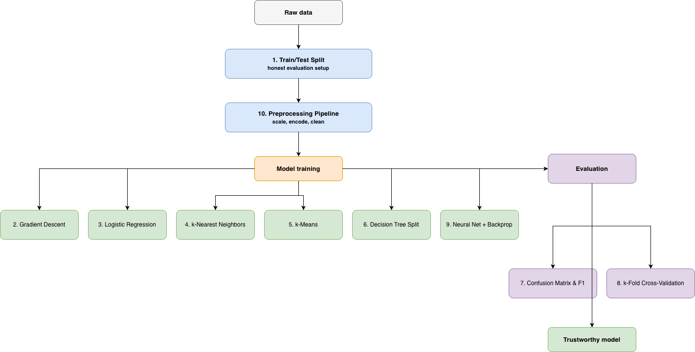
You don’t need to write them in this order. But seeing where each one lives explains why they’re the must-know ten and not ten randomly chosen algorithms.

1. A reproducible train / validation / test split

Everyone thinks they understand this one, and then they leak data anyway. Writing the split yourself — with a fixed random seed and a clear three-way boundary — forces you to confront the single most common cause of models that look brilliant offline and fall apart live.

import numpy as np

def split(X, y, val=0.15, test=0.15, seed=42):
    rng = np.random.default_rng(seed)
    idx = rng.permutation(len(X))
    n_test = int(len(X) * test)
    n_val = int(len(X) * val)
    test_idx, val_idx, train_idx = idx[:n_test], idx[n_test:n_test+n_val], idx[n_test+n_val:]
    return (X[train_idx], y[train_idx]), (X[val_idx], y[val_idx]), (X[test_idx], y[test_idx])

What it teaches: The test set is sacred — you touch it once, at the very end. The validation set is where you make decisions; the test set is where you find out whether those decisions generalized. The instant you scale features or select columns using statistics computed over the whole dataset, information from the test set has leaked into training, and your score becomes fiction. Writing the split by hand makes that boundary physical instead of theoretical.

2. Linear regression by gradient descent

This is the engine room. Almost every model you’ll ever train — logistic regression, neural networks, gradient-boosted trees in a loose sense — minimizes a loss function by nudging parameters in the direction that reduces error. Write it once and the word “optimizer” stops being a black box.

def gradient_descent(X, y, lr=0.01, epochs=1000):
    w = np.zeros(X.shape[1])
    b = 0.0
    n = len(y)
    for _ in range(epochs):
        preds = X @ w + b
        error = preds - y
        w -= lr * (2/n) * (X.T @ error)   # gradient of MSE w.r.t. weights
        b -= lr * (2/n) * error.sum()      # gradient w.r.t. bias
    return w, b

What it teaches: The learning rate is a genuine trade-off, not a default. Set it too high and the loss oscillates or explodes; too low and training crawls. You feel this immediately when you print the loss each epoch and watch it either descend smoothly or thrash. You also learn that “training” is just this loop, repeated — every fancy optimizer (Adam, RMSprop) is a smarter version of the same two lines.

3. Logistic regression and cross-entropy loss

Linear regression predicts numbers; logistic regression predicts probabilities. The jump between them is small in code but large in understanding: you wrap the linear output in a sigmoid, and you swap mean-squared error for cross-entropy loss.

def sigmoid(z):
    return 1 / (1 + np.exp(-z))

def train_logistic(X, y, lr=0.1, epochs=1000):
    w, b = np.zeros(X.shape[1]), 0.0
    for _ in range(epochs):
        p = sigmoid(X @ w + b)
        w -= lr * (X.T @ (p - y)) / len(y)
        b -= lr * (p - y).mean()
    return w, b

What it teaches: Why we don’t just use accuracy as a loss. Cross-entropy punishes a confident wrong answer far more harshly than a hesitant one, which is exactly the incentive you want — a model that says “99% cat” about a dog should hurt more than one that says “55% cat.” Notice, too, that the gradient update looks almost identical to linear regression’s. That’s not a coincidence; it’s a hint at why the same optimization machinery scales across so many models.

4. k-Nearest Neighbors from scratch

k-NN is the simplest possible classifier: to predict a new point, find the k closest training points and take a vote. It has no training step at all — the entire model is the dataset. That makes it the perfect first baseline and a brutal teacher of one of ML’s hardest lessons.

def knn_predict(X_train, y_train, x, k=5):
    distances = np.linalg.norm(X_train - x, axis=1)
    nearest = np.argsort(distances)[:k]
    labels, counts = np.unique(y_train[nearest], return_counts=True)
    return labels[counts.argmax()]

What it teaches: The curse of dimensionality, viscerally. In two dimensions, “nearest” means something. In five hundred dimensions, every point is roughly equidistant from every other, distances lose meaning, and k-NN quietly degrades to guessing. Watching your k-NN accuracy collapse as you add noise features is a lesson about feature selection that no diagram delivers as convincingly. You also feel why “no training cost” comes at the price of “expensive prediction” — every single prediction scans the whole dataset.

5. k-Means clustering

Move from supervised to unsupervised learning by grouping data with no labels at all. k-Means alternates two steps until it settles: assign each point to its nearest center, then move each center to the average of its assigned points.

def kmeans(X, k=3, iters=100, seed=0):
    rng = np.random.default_rng(seed)
    centers = X[rng.choice(len(X), k, replace=False)]
    for _ in range(iters):
        labels = np.array([np.argmin(np.linalg.norm(x - centers, axis=1)) for x in X])
        new_centers = np.array([X[labels == j].mean(axis=0) for j in range(k)])
        if np.allclose(new_centers, centers):
            break
        centers = new_centers
    return centers, labels

What it teaches: Initialization matters, and local optima are real. Run k-Means twice with different starting centers and you can get two different answers — which is why production implementations (like k-means++) are careful about where they start. You also confront the awkward truth that you have to pick k; the algorithm won’t tell you how many clusters exist. That single decision, and the elbow/silhouette methods people use to make it, teaches more about unsupervised learning than a chapter of prose.

6. A decision-tree split with Gini impurity

You don’t need to build a full recursive tree (though it’s a great weekend project). You need to write the one function at a tree’s heart: given a column and a threshold, how good is this split? Trees are just this decision, made greedily, over and over.

def gini(y):
    _, counts = np.unique(y, return_counts=True)
    p = counts / counts.sum()
    return 1 - (p ** 2).sum()

def best_split(X, y):
    best = (None, None, 1.0)   # (feature, threshold, weighted_impurity)
    for f in range(X.shape[1]):
        for t in np.unique(X[:, f]):
            left, right = y[X[:, f] <= t], y[X[:, f] > t]
            if len(left) == 0 or len(right) == 0:
                continue
            w = (len(left) * gini(left) + len(right) * gini(right)) / len(y)
            if w < best[2]:
                best = (f, t, w)
    return best

What it teaches: How a tree “chooses” — it’s not intelligence, it’s an exhaustive search for the split that makes the resulting groups as pure as possible. Once you’ve written this, random forests and gradient boosting stop being mysterious: they’re just clever ways of combining many of these greedy little decisions to cancel out each other’s mistakes. You also see instantly why a single deep tree overfits — keep splitting and you can drive impurity to zero by memorizing the training data.

7. A confusion matrix and F1 score by hand

Accuracy is the most misleading number in machine learning, and the only cure is to compute what it hides. Build a confusion matrix and derive precision, recall, and F1 from its four cells.

def metrics(y_true, y_pred):
    tp = np.sum((y_true == 1) & (y_pred == 1))
    tn = np.sum((y_true == 0) & (y_pred == 0))
    fp = np.sum((y_true == 0) & (y_pred == 1))
    fn = np.sum((y_true == 1) & (y_pred == 0))
    precision = tp / (tp + fp) if tp + fp else 0
    recall = tp / (tp + fn) if tp + fn else 0
    f1 = 2 * precision * recall / (precision + recall) if precision + recall else 0
    return {"precision": precision, "recall": recall, "f1": f1, "accuracy": (tp+tn)/len(y_true)}

What it teaches: Why a fraud detector that’s 99.9% accurate can be completely useless. If 1 in 1000 transactions is fraud, a model that predicts “never fraud” scores 99.9% accuracy and catches zero criminals. Precision (“when I raise an alarm, am I right?”) and recall (“of all the real cases, how many did I catch?”) expose that failure instantly. Deciding which one matters more — a spam filter wants precision, a cancer screen wants recall — is one of the most consequential judgment calls in applied ML, and this program is where it clicks.

8. A k-fold cross-validation loop

A single train/test split is one roll of the dice. Cross-validation rolls it k times, using each slice of the data as the test set once, and averages the result — giving you an estimate of performance with a sense of how much it wobbles.

def k_fold_cv(X, y, train_fn, score_fn, k=5, seed=0):
    idx = np.random.default_rng(seed).permutation(len(X))
    folds = np.array_split(idx, k)
    scores = []
    for i in range(k):
        test_idx = folds[i]
        train_idx = np.concatenate([folds[j] for j in range(k) if j != i])
        model = train_fn(X[train_idx], y[train_idx])
        scores.append(score_fn(model, X[test_idx], y[test_idx]))
    return np.mean(scores), np.std(scores)

What it teaches: That the variance of your score is as important as its mean. A model that scores 0.85 ± 0.02 across folds is trustworthy; one that scores 0.85 ± 0.15 is telling you the performance depends heavily on which data it happened to see. That standard deviation is an early-warning system for a model that hasn’t really learned a stable pattern — and it’s the number that stops you from over-celebrating a lucky split.

9. A one-hidden-layer neural network with backpropagation

This is the program that demystifies deep learning. A network with a single hidden layer, trained with backpropagation, contains every idea that scales up to a transformer: a forward pass that produces a prediction, a loss that measures the error, and a backward pass that uses the chain rule to figure out how each weight contributed to that error.

def train_nn(X, y, hidden=8, lr=0.1, epochs=2000):
    rng = np.random.default_rng(0)
    W1, b1 = rng.normal(size=(X.shape[1], hidden)) * 0.1, np.zeros(hidden)
    W2, b2 = rng.normal(size=(hidden, 1)) * 0.1, np.zeros(1)
    for _ in range(epochs):
        h = np.tanh(X @ W1 + b1)          # forward: hidden activations
        out = sigmoid(h @ W2 + b2)         # forward: output probability
        d_out = (out - y.reshape(-1, 1)) / len(y)          # loss gradient
        d_h = (d_out @ W2.T) * (1 - h**2)                   # backprop through tanh
        W2 -= lr * h.T @ d_out; b2 -= lr * d_out.sum(0)     # update output layer
        W1 -= lr * X.T @ d_h;   b1 -= lr * d_h.sum(0)       # update hidden layer
    return W1, b1, W2, b2

What it teaches: That backpropagation is not sorcery — it’s the chain rule from calculus, applied mechanically layer by layer. Once you’ve written those two backward lines yourself, loss.backward() in PyTorch stops being magic and becomes “oh, it’s doing what I did, automatically, for a thousand layers.” You also learn why weight initialization matters (start at zero and every hidden unit learns the same thing) and why nonlinear activations like tanh are essential (without them, stacking layers collapses back into a single linear model).

10. A minimal end-to-end pipeline

The final program isn’t an algorithm — it’s the discipline of gluing everything together into something reproducible: load data, preprocess it (scale numbers, encode categories), train, evaluate, and persist the model to disk so it can be loaded again unchanged.

import joblib

def run_pipeline(X, y):
    (Xtr, ytr), (Xval, yval), (Xte, yte) = split(X, y)
    mean, std = Xtr.mean(0), Xtr.std(0) + 1e-8     # fit scaler on TRAIN only
    Xtr, Xval, Xte = (Xtr-mean)/std, (Xval-mean)/std, (Xte-mean)/std
    w, b = train_logistic(Xtr, ytr)
    val = metrics(yval, (sigmoid(Xval @ w + b) > 0.5).astype(int))
    joblib.dump({"w": w, "b": b, "mean": mean, "std": std}, "model.pkl")
    return val

What it teaches: That a model is not just weights — it’s weights plus the exact preprocessing that produced them. Notice the scaler is fit on the training data only, then applied everywhere; save the model without saving mean and std, and your deployed model will silently receive differently-scaled inputs and quietly degrade. This program is the bridge between a notebook that works once and a system that works every day, and it’s the one most self-taught engineers skip — right up until it costs them a production incident.

How to actually use this list

Don’t write all ten in one sitting and tick a box. Write one, then go read that same algorithm’s source in scikit-learn or PyTorch and compare. You’ll notice the library version handles a dozen edge cases yours ignored — numerical stability, sparse inputs, early stopping — and that comparison is where the deepest learning happens. Your version taught you the idea; the library’s version teaches you the engineering.

A reasonable order: start with the split (1) and metrics (7), because honest evaluation underlies everything. Then gradient descent (2) and logistic regression (3) for the optimization core. Add k-NN (4) and k-means (5) for the geometry of data, the decision-tree split (6) and cross-validation (8) for robustness, the neural network (9) to unlock deep learning, and the pipeline (10) to make any of it deployable.

None of these will make you a better engineer just by existing in a folder. But writing them — struggling with the exploding loss, watching k-NN collapse in high dimensions, finally getting backprop to converge — rewires how you read every paper, debug every model, and reason about every result for the rest of your career. That’s the return on ten afternoons.

Next step: Pick number 2, open an empty file, and don’t look at any reference until your loss actually goes down. The frustration is the lesson. Once it converges, you’ll never look at model.fit() the same way again.