“Estimating Home Value: Predicting Housing Prices via Linear Regression”

Why Learn This? Importance & Motivation

Predicting housing prices using linear regression is a classic real-world problem that ties together statistics, machine learning, and domain (real-estate) insight. Some reasons it’s valuable:

• Intuitive & Concrete Application: It gives a tangible application of regression: size, location, bedrooms → price. That helps solidify abstract math.
• Baseline Model: Even when you later use more advanced models (random forest, XGBoost, neural nets), linear regression is a strong baseline and often surprisingly competitive.
• Interpretability: Regression gives interpretable coefficients (e.g. “each extra square meter adds £2000”), which is crucial in real estate decisions and reporting.
• Interview/Exam Frequent Topic: Many data science or machine learning interviews ask you to implement or analyze linear regression in a housing-price toy dataset. Knowing it from both theory and code is a strong plus.
• Statistical Foundation: Understanding least squares, residuals, overfitting, assumptions (linearity, homoscedasticity, independence) builds foundation for more advanced modeling.

Thus mastering this concept helps you in both practical modeling and conceptual understanding for exams or job interviews.

Overview & Roadmap

Here’s how we’ll proceed:

1. Conceptual Theory

   • Simple linear regression & multiple linear regression
   • Ordinary least squares (OLS)
   • Assumptions, error terms, residuals

2. Step-by-step workflow for predicting housing prices

3. Three example programs (for each of key sub-concepts) in (a) Python (scikit-learn), (b) R, (c) from-scratch (matrix algebra)

4. Memory / mnemonic tricks for interviews and exams

5. Merquine diagram (concept map)

6. Summary, pitfalls, tips

1. Conceptual Theory

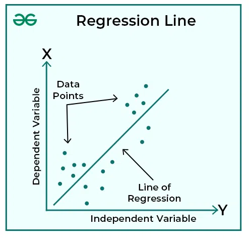
Simple Linear Regression (SLR)

In its simplest form, you try to model:

[ y = \beta_0 + \beta_1 x + \varepsilon ]

• (y) = the dependent variable (e.g. house price)
• (x) = a single independent predictor (e.g. area in sq ft)
• (\beta_0) = intercept (price when x = 0)
• (\beta_1) = slope (how much price increases per unit of x)
• (\varepsilon) = error term (unexplained noise)

We observe data ((x_i, y_i)) for (i = 1,\dots,n). The residual for a data point is:

[ \varepsilon_i = y_i - (\beta_0 + \beta_1 x_i) ]

The “best” estimates (\hat\beta_0, \hat\beta_1) are those that minimize the sum of squared residuals:

[ \min_{\beta_0, \beta_1} \sum_{i=1}^n (y_i - (\beta_0 + \beta_1 x_i))^2 ]

By calculus you derive:

[ \hat\beta_1 = \frac{\sum_i (x_i - \bar x)(y_i - \bar y)}{\sum_i (x_i - \bar x)^2}, \quad \hat\beta_0 = \bar y - \hat\beta_1 \bar x ]

Key points:

• Residuals: vertical distance from point to predicted line
• Goodness: often measured by R², the proportion of variance explained
• Interpretation: (\beta_1) is “price change per 1 unit x”

This is the core of regression. In real housing price problems, though, we rarely have just one predictor.

Multiple Linear Regression (MLR)

To incorporate many features (size, bedrooms, location score, age, etc.), we generalize to:

[ y = \beta_0 + \beta_1 x_1 + \beta_2 x_2 + \dots + \beta_p x_p + \varepsilon ]

In vector/matrix form:

[ \mathbf{y} = \mathbf{X},\boldsymbol{\beta} + \boldsymbol{\varepsilon} ]

• (\mathbf{X}) is the (n \times (p+1)) design matrix (with a column of ones for intercept)
• (\boldsymbol{\beta}) is the ((p+1))-vector of coefficients
• (\boldsymbol{\varepsilon}) is the residual vector

The ordinary least squares (OLS) solution is:

[ \hat{\boldsymbol{\beta}} = (\mathbf{X}^\top \mathbf{X})^{-1} \mathbf{X}^\top \mathbf{y} ]

This formula gives the vector of coefficients that minimize sum of squared errors. This approach is known as the ordinary least squares estimator. ([Wikipedia][1])

Assumptions behind the model:

1. Linearity: relationship between predictors and outcome is linear
2. Independence: errors are independent
3. Homoscedasticity: constant variance of errors
4. No perfect multicollinearity: predictors not perfectly collinear
5. Errors have zero mean and (often) normal distribution (for inference)

Violations of these assumptions can lead to biased or inefficient estimates or invalid inference.

2. Workflow: Predict Housing Prices Using Regression

Here’s a typical step-by-step process when tackling the housing price prediction problem.

(1) Data collection

Gather data with features (predictors) that you think influence price. Example features:

• Size in square feet/meters
• Number of bedrooms
• Number of bathrooms
• Age or year built
• Location / neighborhood index
• Distance to amenities, transport
• Lot size, garden, parking etc.

(2) Exploratory Data Analysis (EDA) & preprocessing

• Check missing values, drop or impute
• Visualize pairwise scatter plots
• Check distributions, outliers, skewness
• Possibly transform features (e.g. log of price)
• Encode categorical features (e.g. one-hot encoding)
• Scale/standardize features (especially if metrics differ widely)

(3) Split data

Divide data into training and test (or train/validation/test). Common splits: 70/30, 80/20.

(4) Fit linear regression model (train)

Using training set, compute coefficient estimates either via library or from-scratch.

(5) Make predictions & evaluate

Use test set to predict prices:

[ \hat y_i = \hat\beta_0 + \sum_j \hat\beta_j x_{ij} ]

Compute performance metrics like:

• Mean Squared Error (MSE)
• Root MSE (RMSE)
• Mean Absolute Error (MAE)
• R² (coefficient of determination)

(6) Diagnostics & residual analysis

• Plot residuals vs predicted values — check for patterns (non-linearity, heteroscedasticity)
• Check for influential points (e.g. high-leverage outliers)
• Check multicollinearity (e.g. via Variance Inflation Factor, VIF)
• Possibly refine model: drop predictors, add interactions or polynomial terms

(7) Final model & deployment

Once satisfied, retrain on full dataset, maybe deploy to production or use for pricing applications.

3. Example Programs (Three per subtopic)

Below are three example programs for regression in the context of housing price prediction. I’ll show:

• (A) Simple regression (one predictor)
• (B) Multiple regression (several predictors)
• (C) From-scratch linear algebra solution

Each in Python, R, and a minimal matrix algebra version.

3A. Simple Regression Examples (one predictor, e.g. size → price)

Python (scikit-learn)

import numpy as np
import pandas as pd
from sklearn.linear_model import LinearRegression
from sklearn.metrics import mean_squared_error, r2_score

# Example data
data = {'size': [50, 70, 90, 110, 130],
        'price': [150_000, 210_000, 270_000, 330_000, 390_000]}
df = pd.DataFrame(data)

X = df[['size']].values  # 2D array
y = df['price'].values

model = LinearRegression()
model.fit(X, y)
y_pred = model.predict(X)

print("Coef (slope):", model.coef_[0])
print("Intercept:", model.intercept_)
print("MSE:", mean_squared_error(y, y_pred))
print("R^2:", r2_score(y, y_pred))

R

# Example data
size <- c(50, 70, 90, 110, 130)
price <- c(150000, 210000, 270000, 330000, 390000)
df <- data.frame(size, price)

model <- lm(price ~ size, data = df)
summary(model)

# predictions
df$pred <- predict(model, newdata = df)
mse <- mean((df$price - df$pred)^2)
r2 <- summary(model)$r.squared
print(mse); print(r2)

From-Scratch (matrix algebra)

Assume arrays:

[ X = \begin{bmatrix} 1 & x_1 \ 1 & x_2 \ \vdots \ 1 & x_n \end{bmatrix}, \quad y = \begin{bmatrix} y_1 \ y_2 \ \vdots \ y_n \end{bmatrix} ]

Compute:

[ \hat\beta = (X^\top X)^{-1} X^\top y ]

In e.g. Python with numpy:

import numpy as np

x = np.array([50, 70, 90, 110, 130])
y = np.array([150000, 210000, 270000, 330000, 390000])
n = len(x)
X = np.vstack([np.ones(n), x]).T  # shape (n, 2)

beta = np.linalg.inv(X.T @ X) @ (X.T @ y)
print("Estimate intercept, slope:", beta)
y_pred = X @ beta
mse = np.mean((y - y_pred)**2)
print("MSE:", mse)

3B. Multiple Regression Examples

Python (scikit-learn)

import numpy as np
import pandas as pd
from sklearn.linear_model import LinearRegression
from sklearn.metrics import mean_squared_error, r2_score

# Example dataset
data = {
    'size': [50, 70, 90, 110, 130],
    'bedrooms': [1, 1, 2, 2, 3],
    'age': [10, 5, 8, 3, 1],
    'price': [150000, 210000, 275000, 335000, 405000]
}
df = pd.DataFrame(data)
X = df[['size', 'bedrooms', 'age']]
y = df['price']

model = LinearRegression()
model.fit(X, y)
print("Coefficients:", model.coef_)
print("Intercept:", model.intercept_)

y_pred = model.predict(X)
print("MSE:", mean_squared_error(y, y_pred))
print("R²:", r2_score(y, y_pred))

R

df <- data.frame(
  size = c(50, 70, 90, 110, 130),
  bedrooms = c(1, 1, 2, 2, 3),
  age = c(10, 5, 8, 3, 1),
  price = c(150000, 210000, 275000, 335000, 405000)
)
model <- lm(price ~ size + bedrooms + age, data = df)
summary(model)
df$pred <- predict(model, newdata = df)
mse <- mean((df$price - df$pred)^2)
r2 <- summary(model)$r.squared
print(mse); print(r2)

From-Scratch (matrix form)

import numpy as np

# Example data
X = np.array([
  [1, 50, 1, 10],
  [1, 70, 1, 5],
  [1, 90, 2, 8],
  [1, 110, 2, 3],
  [1, 130, 3, 1]
])  # (5 samples, 4 columns: intercept + 3 features)
y = np.array([150000, 210000, 275000, 335000, 405000])

beta = np.linalg.inv(X.T @ X) @ (X.T @ y)
print("Beta vector:", beta)
y_pred = X @ beta
mse = np.mean((y - y_pred)**2)
print("MSE:", mse)

3C. Regularized / Diagnostic Variation Example

To illustrate some extensions or diagnostics.

Python: Ridge Regression (to show regularization)

from sklearn.linear_model import Ridge
from sklearn.model_selection import cross_val_score

# reuse X, y from above
ridge = Ridge(alpha=1.0)
ridge.fit(X, y)
print("Ridge coefficients:", ridge.coef_, "Intercept:", ridge.intercept_)
scores = cross_val_score(ridge, X, y, cv=3, scoring='neg_mean_squared_error')
print("CV MSE:", -scores.mean())

R: Stepwise Regression or interactions

# using previous df
model_full <- lm(price ~ size + bedrooms + age, data = df)
model_step <- step(model_full, direction = "both")
summary(model_step)

From-Scratch: Adding interaction term manually

Suppose you want to include an interaction size*bedrooms manually:

import numpy as np

# Create expanded X
size = np.array([50, 70, 90, 110, 130])
bed = np.array([1,1,2,2,3])
age = np.array([10,5,8,3,1])
interaction = size * bed

X = np.column_stack([np.ones(len(size)), size, bed, age, interaction])
y = np.array([150000, 210000, 275000, 335000, 405000])

beta = np.linalg.inv(X.T @ X) @ (X.T @ y)
print("Beta:", beta)
y_pred = X @ beta
print("MSE:", np.mean((y - y_pred)**2))

These examples show how you can extend simple regression to more complex, real-life modeling.

4. How to Remember / Study for Interviews & Exams

To better retain and recall these concepts, here are some strategies:

• Mnemonic “LINEAR”:

  • L — Least squares
  • I — Intercept & slope
  • N — No multicollinearity (assumption)
  • E — Errors (residuals)
  • A — Assumptions (linearity, homoscedasticity etc.)
  • R — R² & Residual analysis

• Flashcards:

  • Card: “Formula for (\hat\beta)” → Answer: ((X^\top X)^{-1} X^\top y)
  • Card: “Assumptions of linear regression”
  • Card: “Interpretation of coefficient in context of housing”

• Whiteboard walk-throughs: In interview prep, practice walking through the derivation of the slope formula for simple regression, or solving a tiny system by hand.

• Teach it: Explain the concept to a peer or write a blog post in simple language; teaching helps retention.

• Diagram mnemonics: Draw the “merquine” / concept map (below) often, review it just before exams.

• Practice questions: Use toy datasets (4–10 points) and compute coefficients by hand or in code; practice diagnosing assumption violations (e.g. residual plots).

• Compare models: When you learn decision trees, random forests, neural nets — always compare them back against your linear regression baseline. This reinforces linear regression each time.

• Understanding vs. memorizing: Focus on why least squares picks that formula, how residuals affect goodness of fit, and when the assumptions fail. That conceptual core helps more than rote memory.

5. Merquine (Concept / Mind Map) Diagram

Below is a conceptual diagram (merquine map) linking the major ideas of linear regression for housing price prediction:

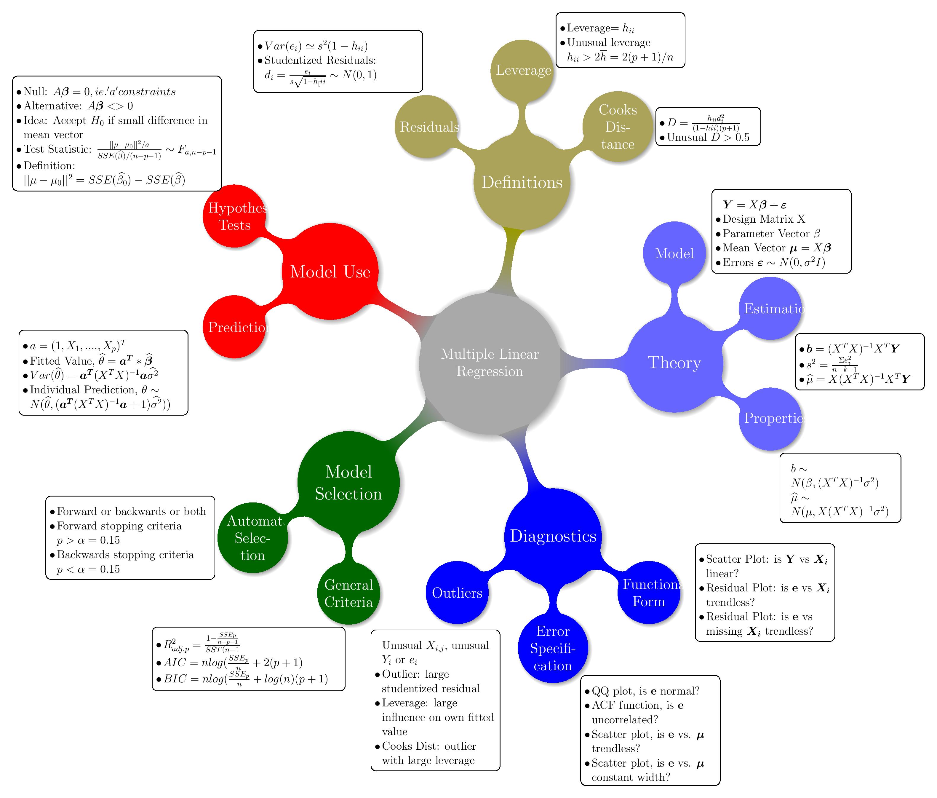
I’ll describe it verbally:

                                +-----------------+
                                |  Housing Price  |
                                +-----------------+
                                         ↑
                              Predict using model y = Xβ + ε
                                         ↑
                +------------------------+------------------------+
                |                                                 |
      +-----------------+                          +----------------------+
      |  Features (X)   |                          |  Coefficients β      |
      +-----------------+                          +----------------------+
      | size, bedrooms, |                          | β0 (intercept), β1, β2... |
      | age, location   |                          +----------------------+
      +-----------------+                                        |
                ↑                                                  |
     Preprocess (encode, scale)                                    |
                |                                                  |
        Data split → train / test                                  |
                |                                                  |
      +----------------------+                            Evaluate on test
      |  Fit by OLS formula  |                            metrics: MSE, R² etc.
      +----------------------+                                 |
                |                                                 |
     Check assumptions & diagnostics                               |
        (residuals, multicollinearity, outliers)                   |
                ↑                                                 |
        Model refinement (interactions, drop features, regularize)

You can sketch this on paper and label arrows to show flow from features → model → predictions → diagnostics → refinement.

6. Summary, Pitfalls & Tips

Summary

• Linear regression models the relationship between independent variables and a dependent variable via a straight line (or hyperplane).
• The OLS method picks coefficients that minimize the sum of squared residuals.
• In housing price prediction, multiple features are usually needed; regression remains a solid, interpretable baseline.
• Implementation is straightforward in Python, R, or even via matrix math.
• Key is to also perform residual diagnostics, check assumptions, possibly regularize or refine model.

Common Pitfalls & Warnings

• Overfitting with too many features: especially if data is small.
• Multicollinearity: predictors that are strongly correlated (e.g. size and number of rooms) can distort coefficients.
• Outliers & high-leverage points: these can disproportionately affect coefficient estimates.
• Violations of assumptions: e.g. heteroscedasticity (variance of residuals not constant), nonlinearity, or autocorrelation.
• Extrapolation danger: model is valid within the domain of training data; predicting outside that (e.g. much larger houses) is risky.
• Interpretation misuse: a positive coefficient doesn’t guarantee causation — only correlation after controlling for included variables.

Tips

• Always baseline with linear regression before jumping to complex models.
• Use cross-validation to guard against overfitting.
• Standardize or normalize variables to make coefficient interpretation easier.
• Use regularization (Ridge, Lasso) if you have many features.
• Use feature selection or PCA if dimensionality is high.
• Always visualize residuals — residual plots often reveal more than summary metrics.
• In interview, accompany your code with discussion of assumptions, diagnostics, limitations.