Data Build Tools
Core Foundations of dbt
- What is dbt
- ELT vs ETL
- dbt Project Structure
- dbt_project.yml
- profiles.yml
- dbt Core vs dbt Cloud
- dbt Environment Management
Models and Materializations
Understanding dbt Models: SQL-based Transformations in Analytics Engineering
In dbt (data build tool), models are the heart of transformation logic. A dbt model is simply a SQL file (or, more recently, a Python model) that describes how to transform raw or upstream data into a cleaned, structured form for analytics. Despite the simplicity, mastering dbt models is essential to build reliable, modular, version-controlled data pipelines.
In this article, we will explore:
- What is a dbt model — definitions, conventions, how dbt treats them
- Core capabilities and configurations (materializations, dependencies, etc.)
- Three example “programs” (SQL model files) for each of several patterns
- A “Merquine-style” flow / architecture diagram
- Memory / exam / interview tips
- Why this concept is important
- Common pitfalls and best practices
Let’s begin by grounding in what exactly a model is in dbt.
What Is a dbt Model?
Definition & basic behavior
- In dbt Core, models are SQL files (with
.sqlextension) stored (typically) in themodels/directory of a dbt project. ([dbt Developer Hub][1]) - Each SQL file must contain a
SELECTstatement (i.e. a query). dbt compiles that into aCREATE TABLE ASorCREATE VIEW AS, depending on the chosen materialization. ([dbt Developer Hub][1]) - The model name is derived from the filename. For example,
models/orders_agg.sqldefines a model calledorders_agg. The model name must exactly match (including case) to avoid issues. ([dbt Developer Hub][1]) - During
dbt run, dbt orders model execution based on dependencies (usingref()calls), compiles each model’s SQL (resolving Jinja, macros, etc.), and then materializes them in the target warehouse. ([dbt Developer Hub][2]) - The compiled SQL (the version actually sent to the warehouse) is stored in the
target/directory so you can inspect it. ([dbt Developer Hub][3])
Thus, dbt models are essentially “declarative SQL statements” wrapped in a managed pipeline.
Why models, not raw SQL scripts?
- Models are versionable, modular, and composable: you can
ref()one model from another, forming a dependency graph. - You can attach configuration, metadata, testing, documentation to models.
- The pipeline abstracts away manual DDL, schema management, table dropping, rename safety, etc.
- You get lineage tracking, easier refactoring, and more maintainable code base.
Supported model types
Although SQL is the primary mode, since dbt v1.3+ dbt also supports Python models — you can write a .py file that defines a function returning a dataframe. ([dbt Developer Hub][4]) But for this article we’ll focus on SQL models because that is the core use case and the foundation for many interviews/exams.
Core Capabilities & Configurations of Models
When defining a dbt model, you don’t just write a SELECT — you can also configure behavior and relationships. Here are key dimensions:
Materializations
Materialization determines how the model is stored in the data warehouse:
- view — model becomes a view
- table — model becomes a full table
- incremental — only new (or changed) data is appended or merged
- ephemeral — the model is never materialized; it’s inlined as a CTE into dependent models ([DEV Community][5])
You configure materialization via the {{ config(...) }} macro or via project-level YAML config.
Dependencies & ref()
- Use
{{ ref('other_model') }}to refer to another model in your project. That ensures dependency ordering, and dbt “knows” to build the referenced model first. ref()also handles schema and naming resolution, so you don’t hardcode full table paths.- Because of
ref(), you can build layered architectures: staging models → intermediate models → marts.
Sources & source()
- To reference raw tables that weren’t created via dbt, you define sources in
.ymlfiles undermodelsorsrcdirectories. - Then, within your model SQL you use
{{ source('source_name', 'table_name') }}instead of literal table names. - This supports freshness checks, metadata, and helps decouple raw name changes.
Additional configuration options
- tags: label models (e.g.
tag: ["staging"]) to select or filter execution. - pre-hooks / post-hooks: SQL statements that run before or after model materialization (e.g. grants, cleanup).
- persist_docs: attach documentation to columns or models.
- enabled / disabled: turn off a model in specific environments.
- partition_by / cluster_by (for warehouses like Snowflake etc.).
- on_schema_change: how to handle when schema of model changes (e.g.
ignore,fail,append).
These configurations can reside inline in your SQL using {{ config(...) }} or in dbt_project.yml or in .yml schema files.
Example Programs / Patterns (3 kinds) for Models
I’ll present three concept categories, each with three example model files.
Pattern Group A: Basic aggregation / transformation models
These are simple transformations: selecting, filtering, grouping.
Example A1: daily_sales_agg.sql
{{ config(materialized="table") }}
with base as (    select        order_id,        order_date::date as dt,        amount    from {{ source('raw', 'orders') }}    where order_status = 'completed')
select    dt,    count(*) as num_orders,    sum(amount) as total_revenuefrom basegroup by dt
This model produces a daily summary of orders and revenue.
Example A2: customer_lifetime_value.sql
{{ config(materialized="incremental", unique_key="customer_id") }}
with cust_events as (    select        customer_id,        event_date,        revenue    from {{ ref('events') }})
select    customer_id,    min(event_date) as first_date,    max(event_date) as last_date,    sum(revenue) as total_revenue,    count(*) as n_eventsfrom cust_eventsgroup by customer_id
Because it’s incremental, new customer events get merged in without rebuilding full table.
Example A3: top_items_by_revenue.sql
{{ config(materialized="view", tags=["analytics"]) }}
select    product_id,    sum(amount) as revenuefrom {{ ref('order_items') }}group by product_idorder by revenue desclimit 50
This is a view showing top revenue-generating products.
Pattern Group B: Layered / modular architecture (staging → intermediate → marts)
Here you build multi-step pipelines, breaking logic into smaller, reusable pieces.
Example B1: stg_orders.sql (staging model)
{{ config(materialized="view", tags=["staging"]) }}
select    order_id,    customer_id,    order_date,    status,    amountfrom {{ source('raw', 'orders_raw') }}
This just cleans raw orders into a canonical staging format.
Example B2: int_customer_orders.sql (intermediate model)
{{ config(materialized="table", tags=["intermediate"]) }}
with orders as (    select * from {{ ref('stg_orders') }}),cust as (    select * from {{ ref('stg_customers') }})select    o.customer_id,    o.order_id,    o.order_date,    c.region,    o.amountfrom orders ojoin cust c using (customer_id)
This model enriches orders with customer metadata.
Example B3: mart_revenue_by_region.sql (data mart)
{{ config(materialized="table", tags=["mart"]) }}
select    region,    sum(amount) as total_revenue,    count(distinct customer_id) as num_customersfrom {{ ref('int_customer_orders') }}group by region
This is a final consumer-facing aggregated table.
Pattern Group C: Conditional / dynamic logic / environment awareness
These models incorporate branching logic (for dev / test / prod or toggles).
Example C1: limited_data_dev.sql
{% set limit_clause = (target.name == 'dev') | ternary("where dt >= current_date - 7", "") %}
{{ config(materialized="table") }}
with base as (    select * from {{ ref('stg_events') }}    {{ limit_clause }})
select    user_id,    count(*) as event_countfrom basegroup by user_id
In dev, you limit to only last 7 days; in prod no limit.
Example C2: dynamic join based on flag
{% set use_latest_dim = var('use_latest_dim', false) %}
{{ config(materialized="table") }}
with events as (    select * from {{ ref('stg_events') }}),dim as (    {% if use_latest_dim %}        select * from {{ ref('dim_customers_latest') }}    {% else %}        select * from {{ ref('dim_customers') }}    {% endif %})
select    e.*,    d.regionfrom events eleft join dim d using (customer_id)
You can toggle which dimension table to use via variable.
Example C3: multi-schema behavior
{% macro target_schema() %}  {% if target.name == 'dev' %}    dev_{{ this.schema }}  {% else %}    {{ this.schema }}  {% endif %}{% endmacro %}
{{ config(materialized="table", schema=target_schema()) }}
select    *from {{ ref('some_model') }}
This model writes to different schema in dev vs prod.
Merquine-Style Diagram / Flow for Models & Dependencies
Here’s a conceptual flow diagram (for how models relate, compile, run, dependencies, layering):

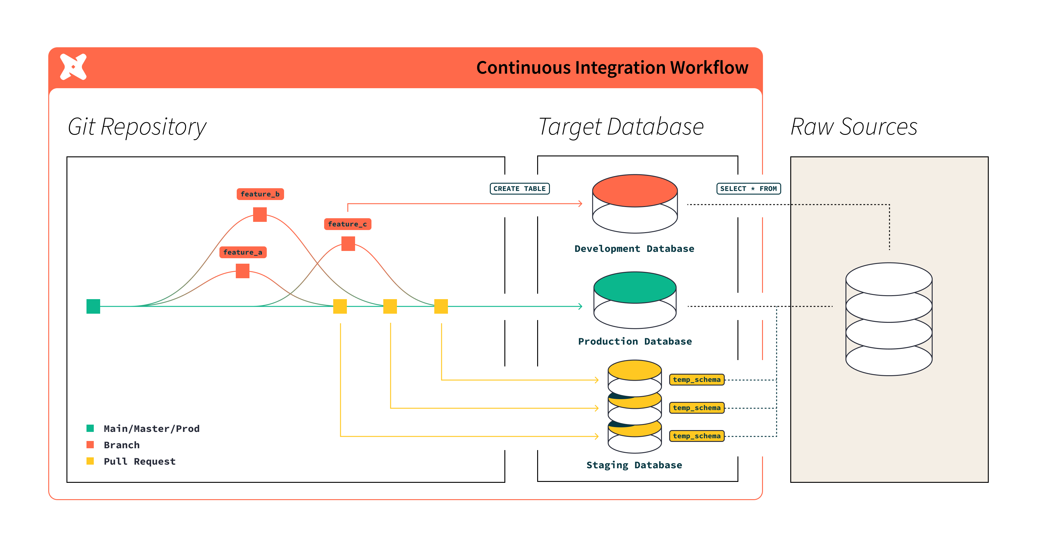
Textual version:
 Sources → [staging models] → [intermediate models] → [mart / data models]
           ↓                     ↓        source.yml           ref() dependencies           ↓                     ↓   dbt compile (resolve SQL) → target/compiled SQL            ↓   dbt run → execution in warehouse            ↓   lineage graph / documentation / tests
Flow explanation:
- Raw data tables are declared as sources.
- Staging models transform raw data into canonical, cleaned formats.
- Intermediate models join or enrich staging data.
- Mart / presentation models produce final analytics.
- dbt uses
ref()to understand dependencies, so it knows build order. dbt compileresolves Jinja, macros, variables, and produces a compiled SQL file intarget/.dbt runexecutes the compiled SQL in the data warehouse, materializing models (views, tables, incremental).- dbt tracks lineage, documentation, and ensures tests / constraints.
This kind of flow is useful to sketch in interviews or on whiteboard to show you understand layers and orchestration.
Memory & Exam / Interview Tips
To solidify your understanding and be able to recall quickly:
-
Mnemonic “STIM”
- Stage (staging)
- Transform (intermediate)
- Integration / join
- Mart (final) Use this to enumerate layering of models.
-
“One SQL per model, one ref per dependency”
- Always think: each
.sql= one model - Use
ref()to connect models
- Always think: each
-
Flashcards
- Q: What is a
.sqlmodel file in dbt? A: A select statement that becomes a table/view (or incremental) after compilation. - Q: What does
materialized="incremental"do? A: Only update or insert new data instead of rebuilding full table. - Q: What is
ref()? A: Function to refer to another model, build dependency graph, resolve naming etc.
- Q: What is a
-
Practice walking through
dbt runstep by step- parse → compile → order → execute → materialize → record metadata
-
Whiteboard exercise
- Draw 3 layers: staging / intermediate / mart
- Label sample model names and draw arrows of dependencies
- Show compiled vs run vs target directory
-
Analogies to software engineering
- Think of staging → intermediate → production layers like “clean modules → business logic → APIs”
- Models are modular functions;
ref()is like function calls
-
Explain aloud to a peer or rubber duck
- Try describing “how dbt transforms a model.sql to a table” step by step
- Explain what happens when you change a model file — how dependencies get recompiled
If asked in an interview, you can mention:
- The structure (
.sql,ref(),config()) - Materializations and how they differ
- Example of layered modeling approach
- Why modular models (testability, maintainability)
- Possibly mention Python models (if interviewer is advanced)
Why It’s Important to Learn dbt Models
Understanding dbt models is critical because:
- Core function: Models are where transformation logic lives. Without models, dbt is just a scaffolding tool.
- Maintainability: Modular models lead to code that’s easier to test, debug, extend, and refactor.
- Version control & collaboration: You can treat models like code, apply code reviews, merge requests, etc.
- Lineage and dependency: Models +
ref()let you build a dependency graph and understand impact of changes. - Performance & cost control: Using incremental models or views selectively can optimize compute usage.
- Testing & documentation: You can attach tests and docs directly to models, improving data quality and visibility.
- Scalability: As your project grows, you need modularization and layering — models enable that.
In short, dbt models are the backbone of analytics engineering. If you don’t master models, you’ll struggle to build robust pipelines.
Common Pitfalls / Best Practices
| Pitfall | Explanation | Avoidance / Best Practice |
|---|---|---|
| Long monolithic SQL files | Hard to read, maintain, debug | Split into staging + intermediate + mart models |
| Hardcoding table/database names | Breaks portability & refactoring | Use source() and ref() instead |
Overuse of config() inline | Scatters config logic | Use project-level YAML where appropriate |
| Incorrect casing in filenames / model names | dbt may not detect or misconfigure | Always match name exactly (underscores, avoid dots) ([dbt Developer Hub][1]) |
Forgetting dependencies / missing ref() | Models run in wrong order or fail | Always reference upstream logic with ref() |
Overuse of view instead of table / incremental | Performance loss or rebuilding repeatedly | Choose materialization appropriate to use case |
| Not inspecting compiled SQL | Complex Jinja logic may miscompile | Use dbt compile to inspect output ([dbt Developer Hub][3]) |
| Schema collisions in development | Multiple devs writing to same schema, interfering | Use schema prefixing macros or dev namespaces |
Summary & Closing
- A dbt model is a
.sqlfile containing aSELECTstatement; dbt compiles it and materializes it as a view, table, or incremental. - Models are composable: using
ref(), you build layered pipelines (staging → intermediate → mart). - Models support rich configuration: materialization, tags, hooks, partitioning, schema overrides.
- Real-world modeling patterns (aggregation, layered design, environment awareness) help structure code.
- The compile → run → lineage flow is central, and you should be comfortable sketching it.
- For interviews, emphasize your understanding of layering, dependency resolution, materializations, and modularity. Use memory aids and whiteboard exercises.
- Knowing models deeply is essential because they are the locus of transformation, maintainability, performance, testing, and scaling of analytics pipelines.